The Sea-Level Change Prediction
The Sea-Level Change Prediction
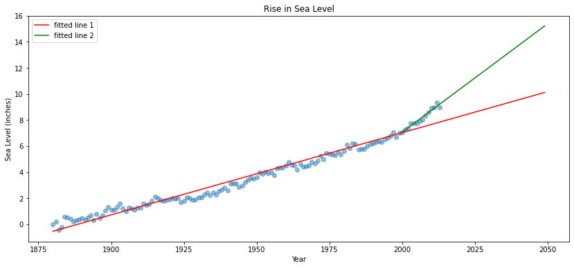
We will analyze the global average sea-level change dataset since 1880 and use the data to forecast sea-level change through the year 2050.
We import the dataset used from https://datahub.io/core/sea-level-rise
Import libraries
import pandas as pd
import matplotlib.pyplot as plt
from scipy.stats import linregress
import numpy as np
!pip -q install datapackage
from datapackage import Package
Download Dataset
package = Package('https://datahub.io/core/sea-level-rise/datapackage.json')
# print list of all resources:
print(package.resource_names)
['validation_report', 'csiro_alt_gmsl_mo_2015_csv', 'csiro_alt_gmsl_yr_2015_csv', 'csiro_recons_gmsl_mo_2015_csv', 'csiro_recons_gmsl_yr_2015_csv', 'epa-sea-level_csv', 'csiro_alt_gmsl_mo_2015_json', 'csiro_alt_gmsl_yr_2015_json', 'csiro_recons_gmsl_mo_2015_json', 'csiro_recons_gmsl_yr_2015_json', 'epa-sea-level_json', 'sea-level-rise_zip', 'csiro_alt_gmsl_mo_2015', 'csiro_alt_gmsl_yr_2015', 'csiro_recons_gmsl_mo_2015', 'csiro_recons_gmsl_yr_2015', 'epa-sea-level']
Global Average Absolute Sea Level Change, 1880-2014
# to load only epa-sea-level_csv dataset
resources = package.resources
resource = resources[5]
df = pd.read_csv(resource.descriptor['path'])
df
| Year | CSIRO Adjusted Sea Level | Lower Error Bound | Upper Error Bound | NOAA Adjusted Sea Level | |
|---|---|---|---|---|---|
| 0 | 1880-03-15 | 0.000000 | -0.952756 | 0.952756 | NaN |
| 1 | 1881-03-15 | 0.220472 | -0.732283 | 1.173228 | NaN |
| 2 | 1882-03-15 | -0.440945 | -1.346457 | 0.464567 | NaN |
| 3 | 1883-03-15 | -0.232283 | -1.129921 | 0.665354 | NaN |
| 4 | 1884-03-15 | 0.590551 | -0.283465 | 1.464567 | NaN |
| ... | ... | ... | ... | ... | ... |
| 130 | 2010-03-15 | 8.901575 | 8.618110 | 9.185039 | 8.122973 |
| 131 | 2011-03-15 | 8.964567 | 8.661417 | 9.267717 | 8.053065 |
| 132 | 2012-03-15 | 9.326772 | 8.992126 | 9.661417 | 8.457058 |
| 133 | 2013-03-15 | 8.980315 | 8.622047 | 9.338583 | 8.546648 |
| 134 | 2014-03-15 | NaN | NaN | NaN | 8.663700 |
135 rows × 5 columns
Prepare Data
df = df[['Year','CSIRO Adjusted Sea Level']]
df = df.dropna(axis=0)
df['Year'] = df['Year'].str.slice(0,4)
df = df.astype({'Year': 'int32'})
df.set_index('Year', inplace=True)
Create scatter plot
# Create scatter plot
plt.figure(figsize=(14,6))
plt.scatter(df.index, df['CSIRO Adjusted Sea Level'], alpha=0.5 )

# Create first line of best fit
res = linregress(df.index, df['CSIRO Adjusted Sea Level'])
year_1880_2050 = np.concatenate((df.index, np.arange(2014,2050)), axis=0)
plt.plot(year_1880_2050 , res.intercept + res.slope*year_1880_2050, 'r', label='fitted line 1')

# Create second line of best fit
res2 = linregress(df.loc['200':].index, df.loc['200':]['CSIRO Adjusted Sea Level'])
year_2000_2050 = np.concatenate((df.loc['200':].index, np.arange(2014,2050)), axis=0)
plt.plot(year_2000_2050 , res2.intercept + res2.slope*year_2000_2050, 'g', label='fitted line 2')

 # Add labels and title
plt.xlabel('Year')
plt.ylabel('Sea Level (inches)')
plt.title('Rise in Sea Level')
plt.legend()